is a solution of the wave equation and is known as d'Alembert's solution, named after the French mathematician Jean le Rond d'Alembert (also educated in law and medicine). 

The two functions and can be determined using the initial conditions 

and  

d'Alembert's Solution 

The solution of the one dimensional wave equation  

,  

with initial conditions 

and for  

and boundary conditions 

and for all  

known as d'Alembert's solution is given by 

where    

and denote the odd extensions of and is some fixed number. 

d'Alembert's Solution 

• pdsolve gives d'Alembert's solution of the wave equation given by

• dAlembert animates d'Alembert's solution of the wave equation during the time . is the number of frames

Example 3 

a) Derive d'Alembert's solution by determining the two arbitrary functions in the general solution using the initial conditions and  

b) Solve the one-dimensional wave equation with for a string of length with zero initial velocity and a profile given by 

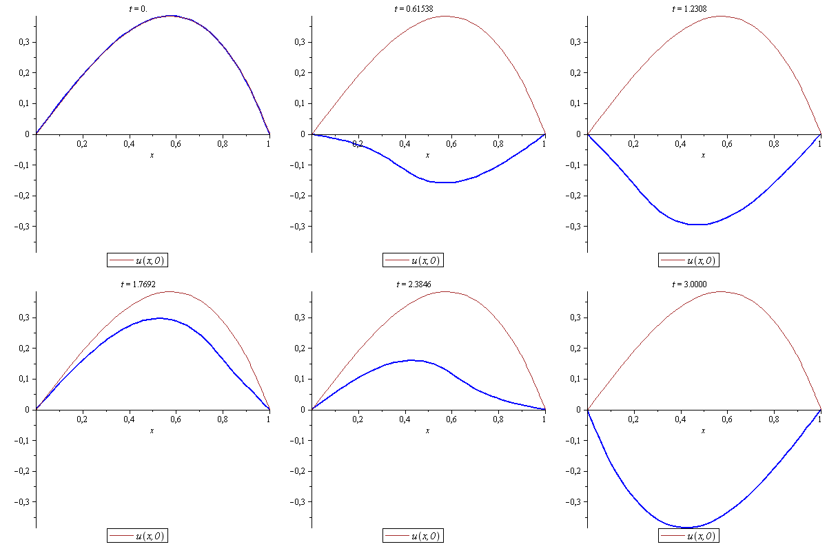
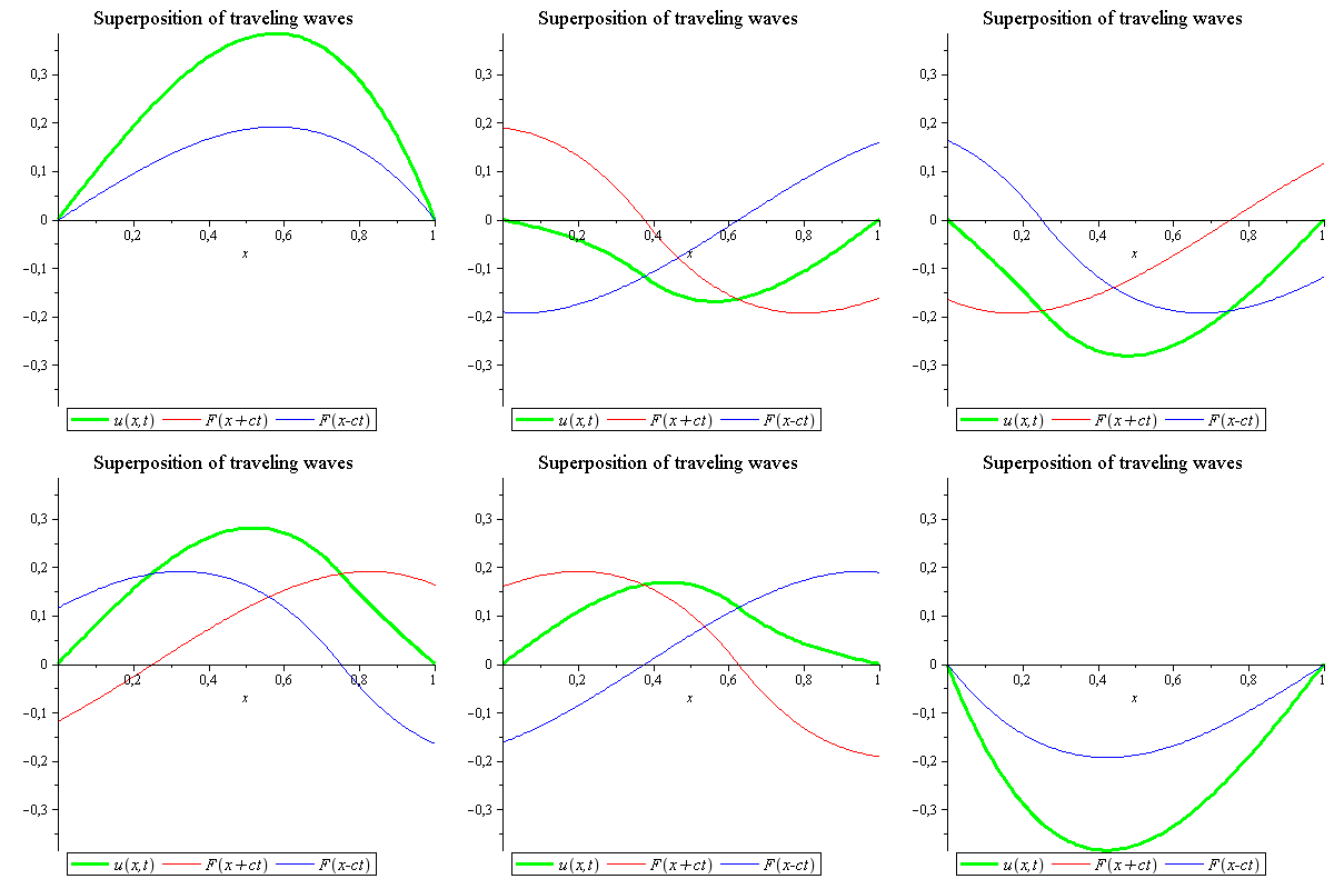
Illustrate the motion of the string by animation and compare it by d'Alembert's solution. 

Solution 

>	restart:MathMaple:-ini():

 

a) The wave equation is   > pde:=diff(u(x,t),t$2)=c^2*diff(u(x,t),x$2):%;	The d'Alembert's solution is  > pdesol:=pdsolve(pde,u(x,t)):%;
> pdesol:=subs(_F1=F[1],_F2=F[2],%):%;	> uxt:=unapply(rhs(pdesol),x,t):   > u(x,t)=uxt(x,t);
d'Alembert's solution satisfying the initial conditions  > eq1:=uxt(x,0)=f(x):%;	> eq2:=D[2](uxt)(x,0)=g(x):%;
Integrating gives  > Int(lhs(eq2),x)=Int(subs(x=s,rhs(eq2)),s=a..x):%;	> eq3:=value(%):%;     > eq1;
Solving for and   > sol:=solve({eq1,eq3},{F[1](x),F[2](-x)}):%;     > F1:=unapply(subs(sol,F[1](x)),x): F2:=unapply(subs(sol,F[2](-x)),x):   The solution of   > pde;     is then  > u(x,t)=F1(c*t+x)+F2(c*t-x);     > expand(%);
b) The solution is given by  > f,g,L,c:=x-x^3,0,1,1;     > u(x,t)=VibratingString(f,g,L,c,infinity): simplify(%) assuming n::integer;     > uxt:=unapply(VibratingString(f,g,L,c,10),x,t): p1:=plot(uxt(x,0),x=0..1,color=brown,legend=typeset(u(`x,0`))):
> u(0.6,0.2)=evalf(uxt(0.6,0.2));     > u(0.6,0.3)=evalf(uxt(0.6,0.3));     > u(0.6,0.5)=evalf(uxt(0.6,0.5));     > u(0.6,1)=evalf(uxt(0.6,1));	> animate(plot,[uxt(x,t),x=0..1,color=blue,thickness=2],t=0..3,frames=40,background=p1):%;

> dAlembert(f,g,L,c,3,40,s):%;     Click and start the animation.

> u(0.6,1)=s(0.6,1);     The approximated solution above using 10 partial sums was .  Using 100 partial sums, we get  > uxt:=unapply(VibratingString(f,g,L,c,100),x,t): p1:=plot(uxt(x,0),x=0..1,color=brown,legend=typeset(u(`x,0`))):   > u(0.6,1)=evalf(uxt(0.6,1));