Multiple Integration 

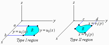
The regions shown in the figure below are called region of type I and region of type II. 

Type I region R:  ,

Type II region R:  ,

If is continuous on a region of Type I (vertically simple), we define an iterated integral of over the region by 

dx 

We first integrate treating in the integrand as a constant. The result of this integration is a function of say Next, integrate . This final result is the value of the iterated integral. The basic idea is to carry out successive integrations. 

In a similar manner, we define an iterated integral of a continuous function over a region of  Type II (horizontally simple) by 

dy = dy 

Iterated integrals provide the means for evaluating a double integral over a region of Type I or Type II or a region that can be expressed as a union of a finite number of these regions. 

Evaluation of Double Integrals 

Let be continuous on a region  

• If is of Type I, then

• If is of Type II, then

dy 

Evaluation of Double Integrals 

• Doubleint (,.. , ..) is an inert form of double integration. Use   value (Doubleint(...) to force Doubleint to evaluate like int .

We can also calculate the iterated integral using 

• int ( int (, ..), ..)

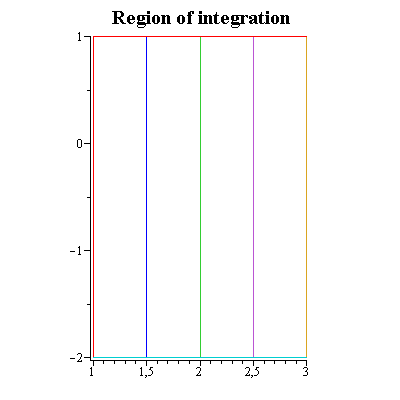
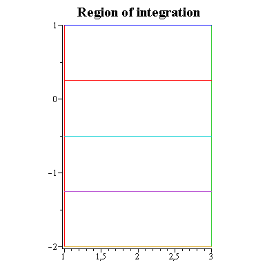
As an aid in reducing a double integral to an iterated integral with correct limits of integration, it is useful to visualize the double summation process pictorially. This can be indicated by vertical lines  in region of Types I and horizontally lines in region of Types II.   

In the package calcplot , you will find commands for plotting such 2D regions described in Cartesian coordinates. 

• dxdyplot () plots the region in the plane with the given arguments as boundary curves

• dydxplot ()  plots the region in the plane with the given arguments as boundary curves

Example 1 

Compute the iterated integrals 

,    

Solution 

a) 

> f:=(x,y)->3*x^4+2*x*y^2;       Region of integration  > dydxplot(y=-2..1,x=1..3,axes=frame,title="Region of integration",titlefont=[times,bold,16]);       The line segments that pass through the interior of the region illustrate elements of integration.   > Ayx:=Doubleint(f(x,y),y=-2..1,x=1..3): Ayx=value(Ayx);

Now we evaluate the integral by reversing the order of integration.  > dxdyplot(x=1..3,y=-2..1,axes=frame,title="Region of integration",titlefont=[times,bold,16]);       We calculate the integral by first integrating from with respect to and then integrating the result from with respect to .  > Axy:=Doubleint(f(x,y),x=1..3,y=-2..1): Axy=value(Axy);