The displacement resonance in forced oscillations
In every oscillating system there is dissipation of mechanical energy, which results that the motion of the mass-spring system described in the previous sections dies out. If the oscillation are to be maintained, energy must be supplied to the system. In this section we shall assume that the system is acted on by a periodic driving force. Suppose that the mass-spring system is subjected to a periodic force ![`*`(F[0], `*`(cos(`*`(omega, `*`(t)))))](images/paper_180.gif) , where
, where ![F[0]](images/paper_181.gif) is the maximum value of the applied force and
is the maximum value of the applied force and  is its frequency. The equation of motion is then
![`+`(`*`(m, `*`(Student:-MultivariateCalculus:-diff(x(t), t, t))), `*`(r, `*`(Student:-MultivariateCalculus:-diff(x(t), t))), `*`(k, `*`(x(t)))) = `*`(F[0], `*`(cos(`*`(omega, `*`(t)))))](images/paper_183.gif)
| > |
 |
| > |
 |
| > |
 |
| > |
 |
| > |
 |
| > |
 |
| > |
 |
The transfer function of the mass-spring system is given by:
| > |
 |
It is easy to show that the steady-state frequency response to an input ![`*`(F[0], `*`(cos(`*`(omega, `*`(t)))))](images/paper_197.gif) becomes
becomes
| > |
![x(t) = `*`(F[0], `*`(abs(('T')(`*`(I, `*`(omega)))), `*`(cos(`+`(`*`(omega, `*`(t)), arg(('T')(`*`(I, `*`(omega)))))))))](images/paper_198.gif) |
| > |
 |
The steady-state system response is also a cosine having the same frequency  as the input.
And the amplitude of this response is ![F[0]](images/paper_203.gif)
 . The variation in both the magnitude
  and argument
  as the frequency
  of the input cosine is varied constitute the frequency response of the system, as the following example shows.
Let us first solve the differential equation using Maples dsolve.
| > |
 |
| > |
 |
| > |
 |
| > |
 |
| > |
 |
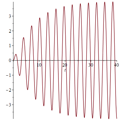
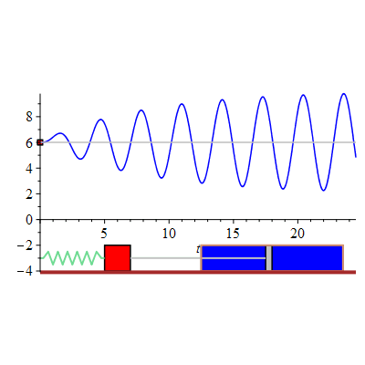
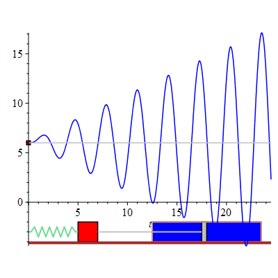
The displacement  of a mass-spring system undergoing forced oscillations plotted against the time with


The graph shows that the transient solution dies out as  increases. The transfer function of the system is given by:
| > |
 |
With 
 and
and  , we get
| > |
 |
| > |
 |
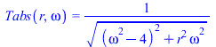
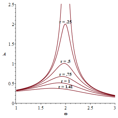
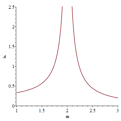
There is some frequency called the resonance frequency at which the amplitude  becomes a maximum. This resonance frequency can be recognized in many vibrating systems unless the damping force
  is too large.
| > |
 |
With zero damping force  the resonance frequency is
The phase angle  is given by
| > |
 |
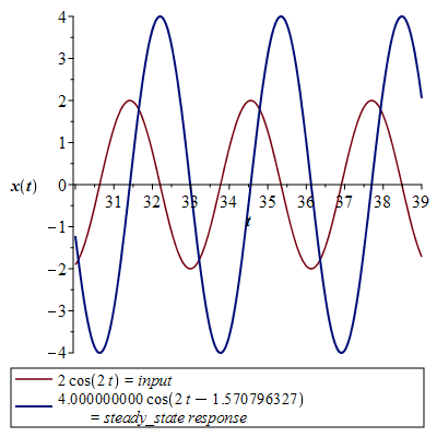
Substituting the values  and
and  gives the steady-state response
| > |
 |
| > |
 |
As 
| > |
 |
| > |
 |
| > |
![plot([f(2, t), xs(t)], t = 30 .. 39, thickness = [1, 2], legend = [typeset(f(2, t) = input), typeset(xs(t) = '`*`(steady_state, `*`(response))')], labels = [t, x(t)], labelfont = [TIMES, BOLD, 12])](images/paper_251.gif)
![plot([f(2, t), xs(t)], t = 30 .. 39, thickness = [1, 2], legend = [typeset(f(2, t) = input), typeset(xs(t) = '`*`(steady_state, `*`(response))')], labels = [t, x(t)], labelfont = [TIMES, BOLD, 12])](images/paper_252.gif) |
| > |
 |
| > |
 |
| > |
 |
| > |
![text2 := proc (i) options operator, arrow; plots:-textplot([2, Tabs(i, 2), convert(r = i, string)], align = ABOVE, font = [TIMES, BOLD, 12]) end proc; -1](images/paper_257.gif) |
| > |
![plots:-display(seq(plt2(i), i = [.1, .25, .5, .75, 1, 1.41]), labels = [omega, A], labelfont = [TIMES, BOLD, 12])](images/paper_258.gif) |
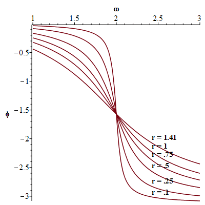
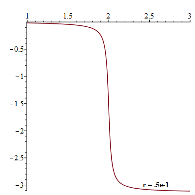
Phase shift between steady-state response and input displacement.
| > |
![plots:-display(seq(plt2(`+`(`*`(0.5e-1, `*`(i)))), i = 1 .. 28), insequence = true, labels = [omega, A], labelfont = [TIMES, BOLD, 12])](images/paper_260.gif) |
Animation
| > |
 |
| > |
![text3 := proc (i) options operator, arrow; plots:-textplot([2.4, phi(i, 2.4), convert(r = i, string)], align = {ABOVE, RIGHT}, font = [TIMES, BOLD, 12]) end proc; -1](images/paper_263.gif) |
| > |
 |
| > |
![plots:-display(seq(plt3(i), i = [.1, .25, .5, .75, 1, 1.41]), labels = [omega, phi], labelfont = [TIMES, BOLD, 12])](images/paper_265.gif) |
Variation of the phase shift  against the angular velocity
| > |
![plots:-display(seq(plt3(`+`(`*`(0.5e-1, `*`(i)))), i = 1 .. 28), labelfont = [TIMES, BOLD, 12], insequence = true)](images/paper_269.gif) |
Animation
| > |
 |
| > |
 |
The displacement of the mass-spring system undergoing forced oscillations with damping constant 
| > |
 |
The displacement of the mass-spring system undergoing forced oscillations with damping constant 
![x(t) = `/`(`*`(F[0], `*`(cos(`+`(`*`(omega, `*`(t)), arg(`/`(1, `*`(`+`(`-`(`*`(m, `*`(`^`(omega, 2)))), `*`(I, `*`(r, `*`(omega))), k)))))))), `*`(abs(`+`(`-`(`*`(m, `*`(`^`(omega, 2)))), `*`(I, `*`(...](images/paper_201.gif)