The response of a mass-spring system to an impulse function
As said above the Dirac delta function could serve as a mathematical model for an external force of large magntiude that acts for only a very short period of time..
| > |
 |
where
| > |
 |
Obviously no real function can satisfy beeing zero except at a single point and have an integral equal to one.
In Maple  is expressed as the derivative of the Heaviside standard unit step function.
| > |
 |
| > |
 |
It is instructive to use Maple to model such an instantaneous unit impulse by starting with the function
| > |
)) = piecewise(`<`(t, a), 0, `<`(t, `+`(a, epsilon)), `/`(1, `*`(epsilon)), 0)](images/paper_151.gif) |
| > |
 |
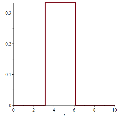
A plot of the rectangular pulse for  and
and  gives
gives
| > |
 |
The area of the rectangular pulse is equal to 1.
| > |
 |
| > |
 |
| > |
 |
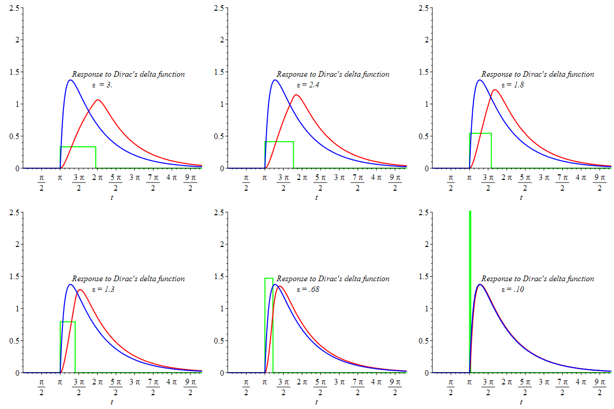
where  is Heavisides unit step function. We can compare the response of a damped mass-spring system to a rectangular pulse
 ))](images/paper_164.gif) as
as  with the response of the Dirac's delta function used by Maple.
The output of the Maple code impulse_func (written above) animates the response to the rectangular pulse ))](images/paper_166.gif) by a linear second order differential equation with constant coefficients and with damping.
by a linear second order differential equation with constant coefficients and with damping.
| > |
 |
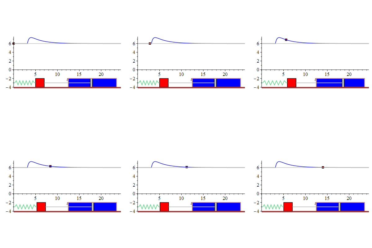
Animation
The behavior of the response to a rectangular pulse by a linear second order differential equation with damping as  compared to the response to Dirac's delta function.
The last animated frame shows little difference between the two responses when 
| > |
 |
| > |
 |
The figure shows an animated response of the damped mass-spring system initially at rest. At time  the system is suddenly given a sharp "hammerblow" modelled by

![]() is expressed as the derivative of the Heaviside standard unit step function.
is expressed as the derivative of the Heaviside standard unit step function. )) = piecewise(`<`(t, a), 0, `<`(t, `+`(a, epsilon)), `/`(1, `*`(epsilon)), 0)](images/paper_152.gif)
![]() and
and ![]() gives
gives 

![]() is Heavisides unit step function. We can compare the response of a damped mass-spring system to a rectangular pulse
is Heavisides unit step function. We can compare the response of a damped mass-spring system to a rectangular pulse ![]() as
as ![]() with the response of the Dirac's delta function used by Maple.
with the response of the Dirac's delta function used by Maple.
![]() by a linear second order differential equation with constant coefficients and with damping.
by a linear second order differential equation with constant coefficients and with damping. 
![]() compared to the response to Dirac's delta function.
compared to the response to Dirac's delta function. ![]()

![]() the system is suddenly given a sharp "hammerblow" modelled by
the system is suddenly given a sharp "hammerblow" modelled by ![]()